Getting started with NumWorks (Statistics)
Calculations Graphing Boxplots Histograms Regression
Objective
The objective of this activity is introduce the NumWorks graphing calculator.
This year we will be using the NumWorks graphing calculator in our math class! This activity will help you get to know the calculator and some of the features we will be using in this class.
The keyboard
Before we get started, let's take a closer look at the keyboard. You'll see it is arranged into three different zones.
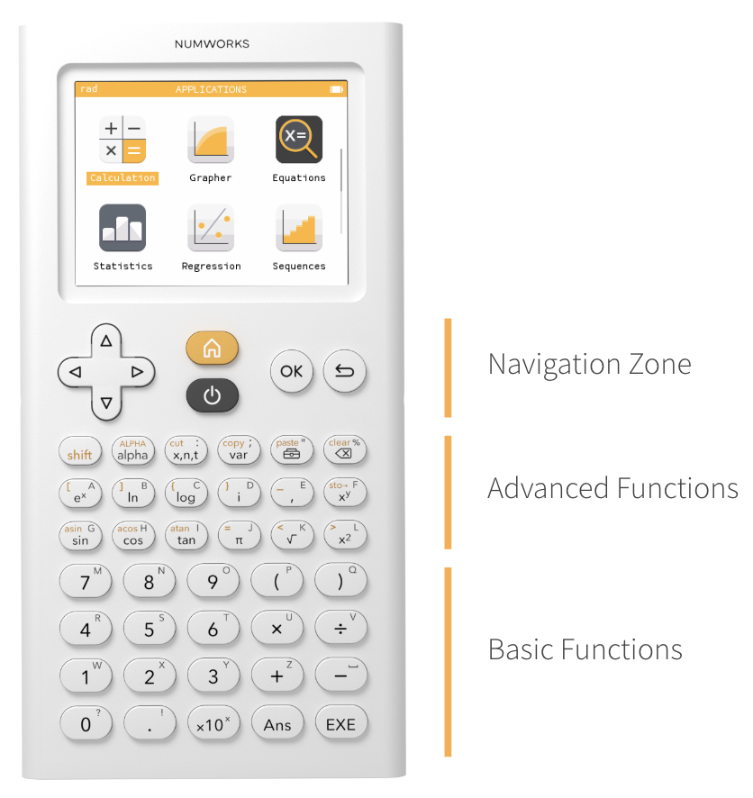
In the bottom section, you will find basic operations and the number pad. Notice that there is only one minus key. Here you will also find the Ans key which allows you to use the most recent result in your calculations. To compute a calculation, press the EXE key.
In the middle section, you will find some advanced functions and commonly used values. What keys do you recognize in this section?
In the top row of the Advanced Functions section, you will find the shift key which gives you access to the yellow option of each key. The alpha key can be used select the alpha characters on each key. The xnt key is a quick way to enter (or other variables as needed). The var key opens a menu of stored values. The Toolbox Toolbox provides additional functions organized in categories. Finally, the Backspace key works just like on your computer or phone to backspace.
The top section is the Navigation Zone where you have arrow keys to navigate the screen, the OK key to make selections and a Back key to take you back to a previous menu. The Home button will return you to the home screen and the Power button turns the calculator on and off.
Navigate around the home screen. How many applications are there?
The applications
The NumWorks calculator is app-based, just like a phone. That means you will open different applications based on the task you are completing. Let's dive into some of the apps to see what they do!
Calculation
![]()
The Calculation application is where you will do all of your... calculations!
Navigate to the Calculation application and open it by pressing OK.
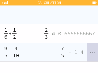
- Let's add some fractions! By hand, add .
- Check your work by using the calculator. What do you notice about your answer?
- Use your calculator to subtract .
- How do the results of the last two calculations differ?
- Navigate up into the calculation history and click on the three dots on the right side of the screen to view the additional results. What additional results are provided for this calculation?
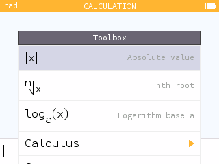
- Return to the editing bar and open the Toolbox. Navigate through the Toolbox and list any functions that you know.
- How many ways are there to select four plants out of the six that are available? Within the Toolbox toolbox, open the Probability section and select Combination. Input .
To input , press the one key followed by the division key. Then press the six key. Use the right arrow key to get out of the denominator before adding the other fraction.
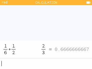
The calculator provides both the simplified fraction and decimal approximation.
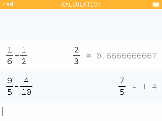
For the first calculation, the decimal result was an approximation and the "approximately equal to" symbol was used. In the second calculation, the decimal result was exact and the "equal to" symbol was used.
Use the up arrow key to navigate into your calculation history. Navigate over to the three dots and press OK.
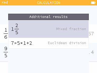
The additional results for include the mixed fraction and Euclidean division representations.
Press the Back key until you return to the editing bar. Open the Toolbox by pressing the toolbox key.
Student responses will vary.
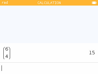
There are 15 ways to select 4 plants out of 6.
Grapher
![]()
Graphing relations and functions is simple within the Grapher application.
Our goal will be to graph the linear function , look at its features and view the table.
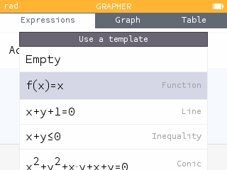
Notice that there are three tabs at the top of the screen: Expressions, Graph and Table.
The Expressions tab is where you will enter your function.
- Press OK to Add an element. There are some templates you can use when entering expressions. For this example, select the template.
- Input the function .
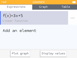
To enter the function , first use the left key to move your cursor to the left of the and add the coefficent . Now use the right key and finish the expression. Once your function is completed, press OK or EXE.
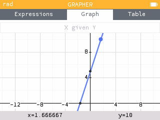
The Graph tab will plot the graphs of your equations and functions and provide tools for exploring key characteristics.
- View the graph. The auto zoom generally provides a window that you will find useful.

To view the graph, either navigate down to Plot graph or up and over to the Graph tab and press OK.
- Press the plus and minus keys to zoom in and out.
- Navigate to . What is the value of ?
Use the left and right keys to trace the line.
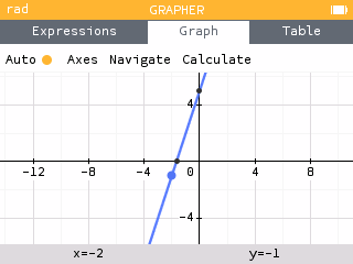
When , .
- What is the value of when ?
Press the four key followed by OK as a shortcut to quickly navigate to .

When , .
- Open the Calculate menu. Then open the Find menu. This menu provides tools for finding key characteristics of our graph. Use the Inverse image option to determine the value of when
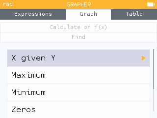
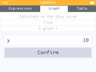
When , .
The Table tab provides a table of points for your function.
- Open the Table tab.
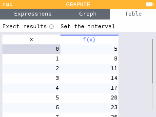
- The table displays the and values for through . Copy down the values of in the table below.
x 0 1 2 3 4 5 6 7 8 9 10 f(x) x 0 1 2 3 4 5 6 7 8 9 10 f(x) 5 8 11 14 17 20 23 26 29 32 35 - What is the value of when ?
Highlight any of the current x-values and type . Press EXE. You will now see the value of in the table.
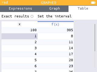
When , .
Statistics
![]()
The Statistics application is great for studying graphical representations of data sets and viewing summary statistics
Open the Statistics app and notice the three tabs at the top of the screen: Data, Graph and Stats.
The Data tab is where you will enter your data.
The table below shows the number of text messages sent in the past 24 hours by the students in a class.
| 0 | 7 | 1 | 29 | 25 | 8 | 5 | 1 | 25 | 98 | 9 | 0 | 26 | 8 | 118 | 72 | 0 | 92 | 52 | 14 | 3 | 3 | 44 | 5 | 42 |
- On the Data tab, enter the values into the V1 column. What do you think N1 represents?
- Once your data is entered, navigate back up to the top of the column and press OK to open the V1 column options. Sort your data.
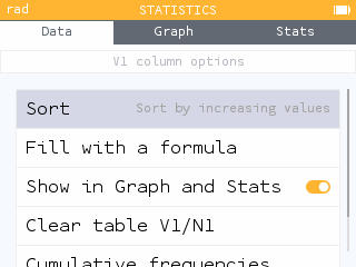
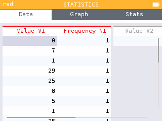
N1 represents the frequencies. It will default to .
To view graphical representations of your data, you will use the Graph tab.
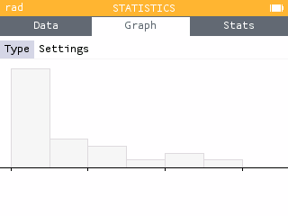
- Open the Graph tab and create a histogram for this data.
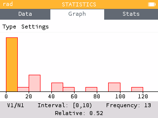
- Navigate through the histogram.
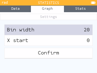
- The histogram is showing "bins" of size 10. Change the Bin width to 20 using the histogram Settings. What do you notice about the distribution?
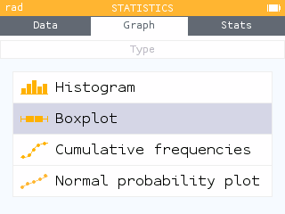
- You can also view a boxplot of the data on number of texts sent. Change the graph from a histogram to a boxplot using the Type menu.
- Navigate through the boxplot. Record the values shown in the bottom banner.
- The last value in the boxplot is displayed as a single dot. What does this represent about that data point?
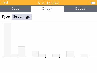
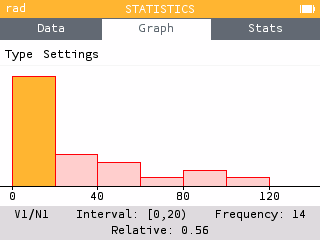
Most of the data appears closer to 0 but a few students send a lot of texts (skewed right).
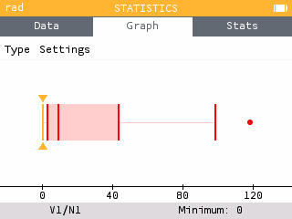
The bottom banner provides the 5-number summary:
| Minimum | First quartile | Median | Third quartile | Upper whisker | Maximum |
| 0 | 3 | 9 | 43 | 98 | 118 |
This data point is an outlier.
The Stats tab provides summary statistics for the dataset.
- Open the Stats tab. What do you notice about the first few entries on this tab?
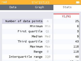
- Scroll through the list of summary statistics found on the Stats tab. Which of the terms or symbols do you recognize?
The first few values match the values found in the bottom banner of the boxplot.
Student answers will vary. Make note of the difference between statistics for a population (mean, standard deviation, variance) and those for a sample (sample mean, sample standard deviation, sample variance).
Regression
![]()
The Regression application plots scatterplots and provides the line of best fit.
Open the Regression application. The Regression app also has three tabs at the top of the screen: Data, Graph and Stats.
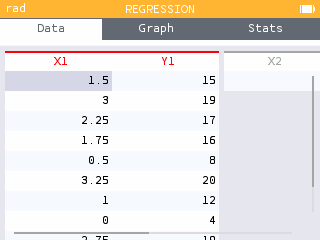
The table below shows the relationship between quiz scores (out of 20) and study time (in hours) for a few students in a class.
| Study time (hours) | 1.5 | 3 | 2.25 | 1.75 | 0.5 | 3.25 | 1 | 0 | 2.75 |
| Score (out of 20) | 15 | 19 | 17 | 16 | 8 | 20 | 12 | 4 | 19 |
- On the Data tab, enter the values of "Study time" into the X1 column and the values of "Score" into the Y1 column.
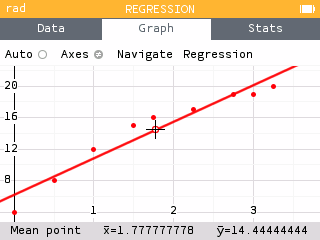
- Select the Graph tab to view the scatterplot.
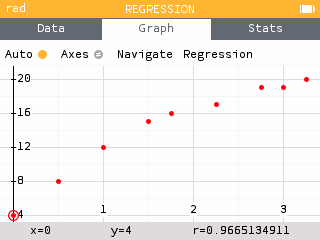
- Navigate through the data points. Notice that the values of and appear in the bottom banner.
- How would you describe the relationship between Study time and Score?
There appears to be a positive, linear relationship. The more time a student studies, the higher their quiz score is.
Let's find the line of best fit.
- While viewing the scatterplot on the Graph tab, press OK to open the list of regression models and select Linear.
- Navigate through the data points and onto the line of best fit. What is the regression equation (round to the nearest hundredth)?
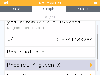
- Find the equation of the line of best fit in the Regression menu.
Press the Toolbox key to open the Regression menu and find the equation of the line.
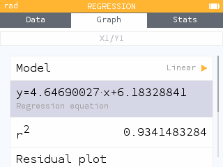
Use the left and right keys to navigate through the data points. While on a data point, use the up or down keys to navigate onto the line of best fit.
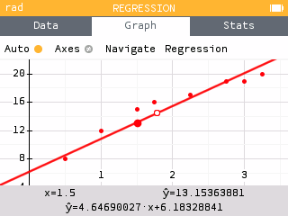
The equation of the line of best fit is
We can use the equation of the line to make predictions for scores based on other study times.
- While in the Regression menu, select Predict Y given X.
- Predict the quiz score for a student who studied for 2 hours.
Enter for .

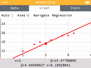
A student who studies for 2 hours is predicted to score a 15.48 on average.
- Return to the Regression menu and select Find X given predicted Y.
Use the back key to return the the Regression menu.
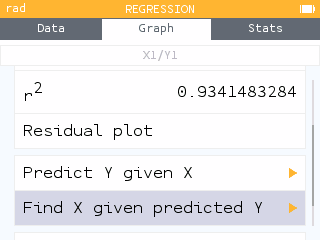
- Determine how many hours of studying a student would need in order to earn a score of 18 on the quiz.
Enter for .
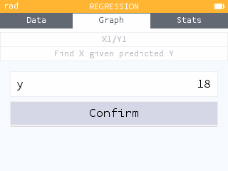
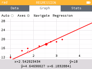
It is predicted that to earn an 18, a student must study for 2.54 hours, on average.
The Stats tab provides summary statistics for our dataset.
- Navigate to the Stats tab and find the row Mean . This reports the mean or average for X1 and Y1.
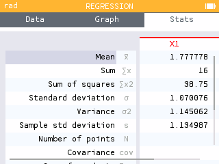
- What is the average amount of time these students studied (round to the nearest hundredth)?
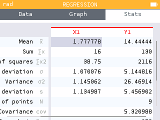
The average amount of time studied by these students is 1.78 hours.
- What is the average quiz score for these students (round to the nearest hundredth)?
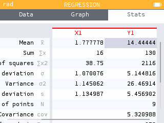
The average score made by these students is 14.44.
Keep exploring!
There's a lot more you can do on the NumWorks calculator! Keep exploring the applications and check out the short tutorials at num.works/tutorials.