The automatic zoom

Have you ever wondered how your calculator “chooses” the axes for your graph? Before our software update 15.3.0, the curves of your functions were well displayed. However, the zoom used was sometimes imperfect. To solve this problem, we had to develop an algorithm capable of calculating a benchmark adapted to each function.

Scale issues

A grapher is a powerful educational tool, particularly for a student new to mathematics. It helps them become familiar with concepts of analysis and to discover the properties of different types of functions. Imagine a student that would like to explore the variations of the function f(x) = x(x-1)(x-3). After entering the expression in the Functions application of the NumWorks calculator, if using version 14 the following would appear:

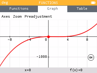
With this visualization, the student would infer that the curve is always increasing with a single root at zero. Lucky for us, this student paid attention during math class! She knows that this is not a monotonic function. However, why did her calculator show her otherwise?

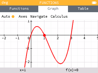
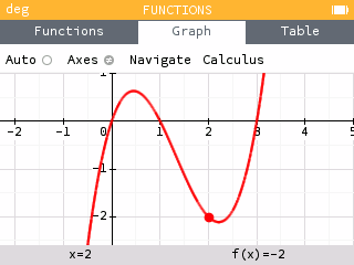
The grapher is not incorrect, but the chosen zoom does not make visible the third degree polynomial. It would be a much clearer picture if the curve was shown like this:

An algorithm that was a little too simple

The question must now be asked: how did the calculator choose a sub-par window when displaying the curve? It all comes down to the algorithm. Before version 14, the algorithm that determined the graphing window was simple. Under this algorithm, the horizontal axis was always -10 to 10 and the vertical axis was selected to provide the best view of the curve.

In the first image, the limits of the y-axis are extreme values of the curve. In this case they are: f(-10)=-1430 and f(10)=630. The local extrema of the function have values of the order of extremity, so it is not surprising that they are invisible.

In software version 15, we decided to update our grapher so that it could zoom in on curves in a more intuitive way. This would be a difficult undertaking, because the underlying question is subjective: what makes one portion of a curve more interesting than another? And above all, how do we translate this notion into mathematical language?

First, we compiled a list of common functions and the zoom that the user would expect for each. This list allowed us to support our solution and make sure that the zooms proposed did not deviate much from the ones we were looking for.

As shown in the first example, the best window often focuses on variations of the curve. With this as a starting point, we can list different points of interest we wish to display on the screen: roots, minima and maxima, vertical and horizontal asymptotes.

Looking for points of interest

The first step in constructing a reference window for the display of a Cartesian curve is to find the points of interest in the function.

For some types of curves, the search for roots or extrema is a problem that is already solved, especially in the case of polynomials of low degree. But in general, there is no formal method of solving the problem. Therefore, we will be satisfied with an approximate solution.

One might think that this question is well documented, and the literature is indeed abundant on the subject of finding roots or extrema in a given finite interval. But, information is harder to come by when this interval is a set of real numbers.

It is typical for a root or extrema search algorithm to go through the interval by calculating values of the function at regularly spaced x coordinates. By comparing consecutive values, we can determine whether the function changes sign or direction of variation. To adapt this strategy to a set of real numbers, we use a geometrical progression rather than arithmetic. This idea is based on the following observation: for most of the functions we have encountered, the distance between two interest points is often of the same order of magnitude as the x coordinates of the interest points themselves. We can now quickly study the function around zero and explore its variations for large x coordinates.

For function f(x)=x(x-1)(x-3), we find five points of interest (three roots and two local extrema), all contained in the interval [0,3]. We add a margin to better center the curve, which gives a horizontal interval around [-2,5]

The second dimension

The second step is to determine the interval displayed on the y-axis.

To begin, we look to see if it is possible to create a more natural orthonormal frame. Since we already know the horizontal interval and the screen ratio, we can deduce the size of the vertical interval. For function f, if the screen has a ratio of 60%, we need to find a vertical interval of size (5-(-2))x60% or 4.2.

Finally, we must determine its position. To do this, we compute a sample of values of the function and look for the fixed interval which contains the maximum number of these values. We are also checking that the points of interest found previously belong to this interval. We thus construct the orthonormal reference frame, maximizing the space occupied by the curve on the screen.

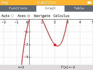
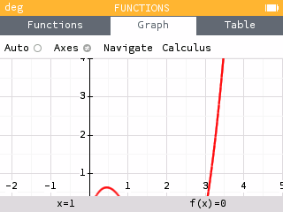
It is not always possible to construct a satisfactory orthonormal reference window. For example, the size of the vertical interval may not be sufficient to display all the points of interest. Consider for example the function 2f, which has the same variations as f. It reaches at its local maximum about 1.3, and at its local minimum about -4.2. It is therefore impossible to display these two values simultaneously with a vertical interval of size 4.2…

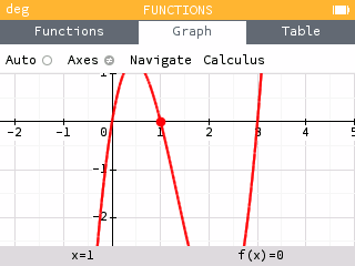
When this occurs, we calculate a measure of the order of magnitude of the function, the average of the logarithm of its absolute value. This quantity indicates whether the function takes its values in the tens, hundreds, thousands, etc. We do not display values that are too large compared to the average order of magnitude. This allows the cutting off the divergent branches of polynomial curves; if they were included in the window, their very rapid growth would crush the rest of the curve. This is what happens in the first example.

A matter of compromise

The automatic zoom algorithm in Epsilon version 15 is considerably more complex than the basic algorithm we have used before, thus it is also more unstable.

A simple algorithm will have predictable behavior, both in its successes and in its failures. When the procedure for displaying a curve is to simply plot all its values between -10 and 10, the algorithm always fails in the same way.

With the new method, the number of bugs, special cases and parameters to choose is multiplied. The path of the horizontal axis can miss an extremum if its step is too large, but can also be too slow if the step is too small. The search for an orthonormal frame of reference can fail if the function is too regular: it cannot choose the best interval since they are all equal. The calculation of the logarithmic mean can be rendered useless if the values of the function are too often zero. Some curves simply have no points of interest and must be reduced to a default interval. The bugs are countless.

The work does not stop there, since the new capabilities of the grapher led us to completely rethink the interface of our Function application!

The final application is a much more practical tool for users, even if the price is a bit more capricious code for us developers.